![]()
![]()
matrixCorr computes correlation and related association
matrices from small to high-dimensional data using simple, consistent
functions and sensible defaults. It includes shrinkage and robust
options for noisy or p >= n settings, plus
convenient print/plot/summary methods. Performance-critical paths are
implemented in C++ with BLAS/OpenMP and memory-aware symmetric updates.
The API accepts base matrices and data frames and returns standard R
objects via a consistent S3 interface.
Contributions from other researchers who want to add new correlation
methods are very welcome. A central goal of matrixCorr is
to keep efficient correlation and agreement estimation in one package
with a common interface and consistent outputs, so methods can be
extended, compared, and used without repeated translation across
packages.
Supported measures include Pearson, Spearman, Kendall, distance correlation, partial correlation, kernel dependence via the Hilbert-Schmidt independence criterion, directed Chatterjee rank correlation, robust biweight mid-correlation, percentage bend, Winsorized, skipped correlation, and latent categorical/ordinal correlations (tetrachoric, polychoric, polyserial, and biserial), plus repeated-measures correlation; agreement tools cover Cohen’s kappa for nominal ratings, weighted Cohen’s kappa for ordered two-rater agreement, Gwet’s AC1/AC2, multi-rater kappa for nominal panel agreement, Krippendorff’s alpha for panel-level reliability, Bland-Altman (two-method and repeated-measures), the coefficient of individual agreement for replicated and repeated-measures designs, Lin’s concordance correlation coefficient (including repeated-measures LMM/REML extensions and Poisson GLMM count-data CCC), and intraclass correlation for both wide and repeated-measures designs.
| Area | Functions and tools |
|---|---|
| Backend | High-performance C++ backend using Rcpp |
| General correlations | pearson_corr(), spearman_rho(),
kendall_tau() |
| Robust correlations | bicor(), pbcor(), wincor(),
skipped_corr() |
| Distance correlation | dcor(), robust_dcor() |
| Kernel dependence | hsic() for raw biased/unbiased HSIC, normalised
kCor-style dependence, kernel bandwidth rules, and permutation
p-values |
| Partial correlation | pcorr() |
| Directed dependence | xi_corr() for Chatterjee rank correlation, with
directed/asymmetric matrices and m-out-of-n bootstrap confidence
intervals |
| Latent categorical/ordinal correlations | tetrachoric(), polychoric(),
polyserial(), biserial() |
| Repeated-measures correlation | rmcorr() |
| Shrinkage for \(p >> n\) | shrinkage_corr() |
| Agreement: two-rater categorical ratings | cohen_kappa() and gwet_ac() for nominal
AC1/AC2 agreement, weighted_kappa() for ordered
categories |
| Agreement: multi-rater and panel reliability | multirater_kappa(), gwet_ac() for panel
AC1/AC2 agreement, krippendorff_alpha() |
| Agreement: Bland-Altman | Two-method or pairwise wide-input ba(),
repeated-measures ba_rm() |
| Agreement: individual agreement | Replicated long-format cia(), repeated-measures
cia_rm() |
| Agreement: probability of agreement | prob_agree() |
| Agreement: concordance | Pairwise Lin’s CCC ccc(), repeated-measures LMM/REML
ccc_rm_reml(), Poisson GLMM count-data CCC
ccc_glmm(), non-parametric ccc_rm_ustat() |
| Agreement: intraclass correlation | Wide-data icc() with pairwise and overall scope,
repeated-measures REML icc_rm_reml() |
| Interactive viewers | Matrix-style Shiny viewers, including the repeated-measures
correlation viewer view_rmcorr_shiny() |
# Install from CRAN
install.packages("matrixCorr")

# Development version from GitHub
# install.packages("remotes")
remotes::install_github("Prof-ThiagoOliveira/matrixCorr")n_threads)Most computational functions expose an n_threads
argument and default to:
getOption("matrixCorr.threads", 1L)To define a package-wide default once per session:
options(matrixCorr.threads = parallel::detectCores(logical = FALSE))library(matrixCorr)
set.seed(1)
X <- as.data.frame(matrix(rnorm(300 * 6), ncol = 6))
names(X) <- paste0("V", 1:6)
R_pear <- pearson_corr(X, ci = TRUE)
R_bicor <- bicor(X)
print(R_pear, digits = 2)
#> Pearson correlation matrix
#> method : pearson
#> dimensions : 6 x 6
#> ci : yes
#>
#> V1 V2 V3 V4 V5 V6
#> V1 1.00 0.02 0.04 -0.02 -0.07 0.01
#> V2 0.02 1.00 0.04 0.03 -0.05 0.13
#> V3 0.04 0.04 1.00 -0.06 0.08 -0.14
#> V4 -0.02 0.03 -0.06 1.00 0.07 0.03
#> V5 -0.07 -0.05 0.08 0.07 1.00 0.04
#> V6 0.01 0.13 -0.14 0.03 0.04 1.00
summary(R_pear)
#> Pearson correlation summary
#> output : matrix
#> dimensions : 6 x 6
#> retained_pairs: 15
#> threshold : 0.0000
#> diag : included
#> estimate : -0.1410 to 0.1272
#> ci : 95%
#> ci_method : fisher_z
#> ci_width : 0.222 to 0.226
#> cross_zero : 13 pair(s)
#>
#> item1 item2 estimate n_complete lwr upr fisher_z statistic p_value
#> V3 V6 -0.1410 300 -0.2502 -0.0282 -0.1419 -2.4459 0.0144
#> V2 V6 0.1272 300 0.0142 0.2371 0.1279 2.2047 0.0275
#> V3 V5 0.0776 300 -0.0360 0.1892 0.0778 1.3401 0.1802
#> V4 V5 0.0724 300 -0.0412 0.1841 0.0725 1.2491 0.2116
#> V1 V5 -0.0650 300 -0.1770 0.0486 -0.0651 -1.1222 0.2618
#> ... ... ... ... ... ... ... ... ...
#> V2 V4 0.0335 300 -0.0801 0.1462 0.0335 0.5773 0.5638
#> V4 V6 0.0324 300 -0.0811 0.1451 0.0324 0.5584 0.5766
#> V1 V2 0.0236 300 -0.0899 0.1365 0.0236 0.4064 0.6845
#> V1 V4 -0.0185 300 -0.1315 0.0949 -0.0185 -0.3187 0.7500
#> V1 V6 0.0130 300 -0.1004 0.1261 0.0130 0.2243 0.8225
#> ... 5 more rows not shown (omitted)
#> Use as.data.frame()/tidy()/as.matrix() to inspect the full result.
#>
#> Strongest pairs by |estimate|
#>
#> item1 item2 estimate n_complete lwr upr fisher_z statistic p_value
#> V3 V6 -0.1410 300 -0.2502 -0.0282 -0.1419 -2.4459 0.0144
#> V2 V6 0.1272 300 0.0142 0.2371 0.1279 2.2047 0.0275
#> V3 V5 0.0776 300 -0.0360 0.1892 0.0778 1.3401 0.1802
#> V4 V5 0.0724 300 -0.0412 0.1841 0.0725 1.2491 0.2116
#> V1 V5 -0.0650 300 -0.1770 0.0486 -0.0651 -1.1222 0.2618
plot(R_bicor)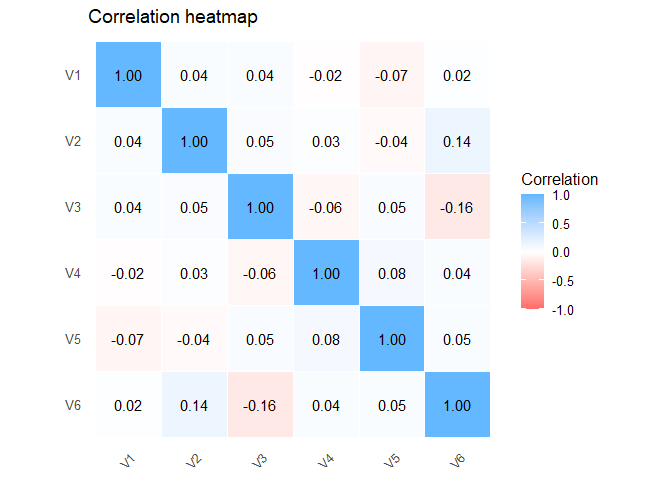
The same matrix-style workflow extends to Spearman, Kendall, distance
correlation, HSIC/kernel dependence, partial correlation, shrinkage
correlation, latent correlation, and the robust estimators
pbcor(), wincor(), and
skipped_corr().
hsic() computes pairwise kernel dependence matrices with
Gaussian, linear, Laplace, and polynomial kernels. It defaults to the
package’s normalised kCor-style output; use
normalise = FALSE to return raw HSIC estimates, and
p_value = TRUE for permutation-based independence
tests.
set.seed(6)
S <- 24
Tm <- 4
id <- factor(rep(seq_len(S), each = 2 * Tm))
method <- factor(rep(rep(c("A", "B"), each = Tm), times = S))
time <- rep(rep(seq_len(Tm), times = 2), times = S)

u <- rnorm(S, 0, 0.9)[as.integer(id)]
um <- rnorm(S * 2, 0, 0.25)
um <- um[(as.integer(id) - 1L) * 2L + as.integer(method)]
y <- u + um + (method == "B") * 0.2 + rnorm(length(id), 0, 0.35)

dat_rm <- data.frame(y, id, method, time)

fit_ccc_rm <- ccc_rm_reml(
  dat_rm,
  response = "y",
  subject = "id",
  method = "method",
  time = "time"
)

summary(fit_ccc_rm)
#>
#> Repeated-measures concordance (REML)
#>
#> Concordance estimates
#>
#>  item1 item2 estimate n_subjects n_obs SB     se_ccc
#>  A     B     0.8328   24         192   0.1096 0.0381
#>
#> Variance components
#>
#>  sigma2_subject sigma2_subject_method sigma2_subject_time sigma2_error
#>  0.7848         0.0192                0.007               0.1168
#>
#> AR(1) diagnostics
#>
#>  ar1_rho ar1_rho_lag1 ar1_rho_mom ar1_pairs ar1_pval use_ar1 ar1_recommend
#>  -0.1073 -0.1073      -0.1073     144       0.198    FALSE   FALSE
Agreement and reliability methods use the same general inspection pattern, but they target different quantities. The package includes Cohen’s kappa for nominal two-rater ratings, weighted kappa for ordered two-rater ratings, Gwet’s AC1/AC2, multi-rater kappa for nominal panel agreement, Krippendorff’s alpha for panel-level reliability, Bland-Altman analysis, concordance correlation, and intraclass correlation for both wide and repeated-measures designs.
The package documentation is organised as a set of workflow vignettes. The README is intentionally brief; the vignettes are the main user guide.
Start here:
vignette("v01-matrixCorr-introduction", package = "matrixCorr")
introduces the package structure, common object behaviour, and shared
display conventions.vignette("v02-wide-correlation-workflows", package = "matrixCorr")
covers Pearson, Spearman, Kendall, distance correlation, and the general
wide-data matrix workflow.vignette("v03-robust-and-highdim-correlation", package = "matrixCorr")
covers robust estimators, shrinkage, and high-dimensional settings.vignette("v04-latent-and-mixed-scale-correlation", package = "matrixCorr")
covers tetrachoric, polychoric, polyserial, and biserial
correlation.vignette("v05-agreement-and-icc-wide", package = "matrixCorr")
covers Bland-Altman analysis, concordance, and intraclass correlation
for wide data.vignette("v06-repeated-measures-workflows", package = "matrixCorr")
covers repeated-measures correlation, repeated agreement, and repeated
reliability workflows.If you want a compact overview of the available estimators, start with the introduction vignette and then move to the workflow family that matches your data layout and scientific question.
Issues and pull requests are welcome. Please see
CONTRIBUTING.md for guidelines and
cran-comments.md/DESCRIPTION for package
metadata.
GPL (>= 3) Thiago de Paula Oliveira
This is a copyleft license: modified versions distributed to others must be distributed under the same GPL terms.