
![]()

![]()
cograph is a modern R package for the analysis, visualization, and manipulation of complex networks. It provides publication-ready plotting with customizable layouts, node shapes, edge styles, and themes through an intuitive, pipe-friendly API. It includes first-class support for Transition Network Analysis (TNA), multilayer networks, and community detection.
# Install from CRAN
install.packages("cograph")

# Development version from GitHub
devtools::install_github("sonsoleslp/cograph")cographNestimate +
cographplot_mcmlsplotqgraph to splot| Function | Description |
|---|---|
splot() |
Base R network plot (core engine) |
soplot() |
Grid/ggplot2 network rendering |
tplot() |
qgraph drop-in replacement for TNA |
plot_htna() |
Hierarchical multi-group TNA layouts |
plot_mtna() |
Multi-cluster TNA with shape containers |
plot_mcml() |
Markov Chain Multi-Level visualization |
plot_mlna() |
Multilayer 3D perspective networks |
plot_mixed_network() |
Combined symmetric/asymmetric edges |
| Function | Description |
|---|---|
plot_transitions() |
Alluvial/Sankey flow diagrams |
plot_alluvial() |
Alluvial wrapper with flow coloring |
plot_trajectories() |
Individual tracking with line bundling |
plot_chord() |
Chord diagrams with ticks |
plot_heatmap() |
Adjacency heatmaps with clustering |
plot_compare() |
Difference network visualization |
plot_bootstrap() |
Bootstrap CI result plots |
plot_permutation() |
Permutation test result plots |
| Function | Description |
|---|---|
overlay_communities() |
Community blob overlays on network plots |
plot_simplicial() |
Higher-order pathway (simplicial complex) visualization |
detect_communities() |
11 igraph algorithms with shorthand wrappers |
communities() |
Unified community detection interface |
| Function | Description |
|---|---|
centrality() |
87 centrality measures, validated against centiserve/sna/igraph/NetworkX |
motifs() / subgraphs() |
Motif/triad census with per-actor windowing |
robustness() |
Network robustness analysis |
disparity_filter() |
Backbone extraction (Serrano et al. 2009) |
cluster_summary() |
Between/within cluster weight aggregation |
build_mcml() |
Markov Chain Multi-Level model construction |
summarize_network() |
Comprehensive network-level statistics |
verify_with_igraph() |
Cross-validation against igraph |
simplify() |
Prune weak edges |
| Function | Description |
|---|---|
supra_adjacency() |
Supra-adjacency matrix construction |
layer_similarity() |
Layer comparison measures |
aggregate_layers() |
Weight aggregation across layers |
plot_ml_heatmap() |
Multilayer heatmaps with 3D perspective |
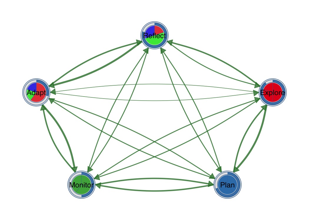
The primary use case: visualize transition networks from the
tna package.
library(tna)
library(cograph)

# Build a TNA model from sequence data
fit <- tna(group_regulation)

# One-liner visualization
splot(fit)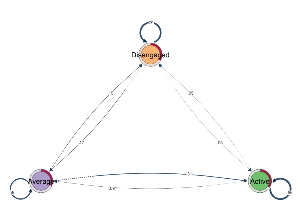
Combine outer donut ring with inner pie segments.
splot(mat,
  donut_fill = fills,
  donut_color = "steelblue",
  pie_values = pie_vals,
  pie_colors = c("#E41A1C", "#377EB8", "#4DAF4A")
)
plot_chord(mat, title = "Transition Chord Diagram")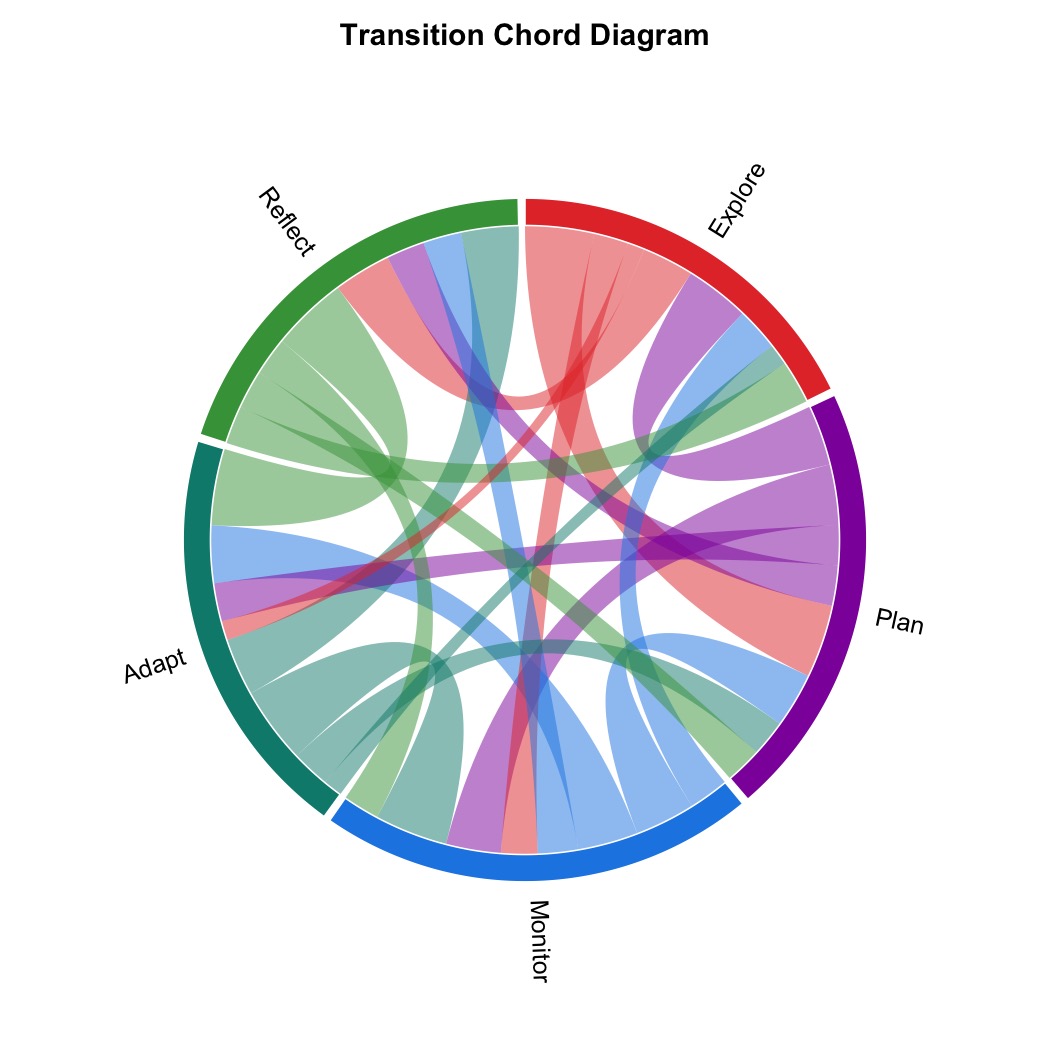
plot_heatmap(mat, show_values = TRUE, colors = "viridis",
             value_fontface = "bold", title = "Transition Heatmap")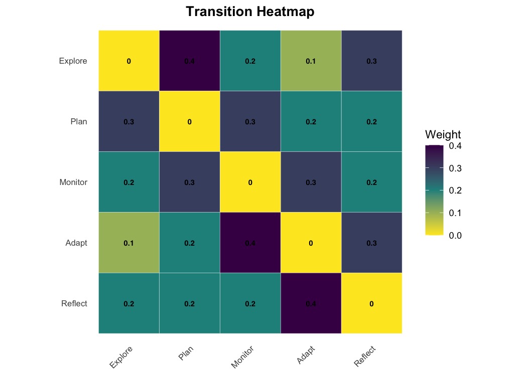
MIT License.